Stabilizing 2D Equations for Physics Informed Networks

Previously on GulfGap, we’ve finished working on 2D Burger’s Equation (which will be released later) during which we’ve started observing instabilities in 2D Equations. In the case of 2D Burger, the network was stabilized by adding a layer before output that enforces boundary conditions using a linear interpolation equation. This layer is called Boundary Encoding Layer.

Sadly, this layer requires careful tweaking of initial conditions and boundary conditions. Altering the conditions for all equations is not ideal for a long-term solution.

After looking through various sources, we’ve solved this by a straightforward solution.

• Rather than returning all output variables through a single layer at the end, each variable now has its own layer.

Why did this work?

In many physics applications, different outputs often represent different physical quantities (for example, velocity vs pressure) that may have different scales, boundary conditions or error sensitivites. When layers are separated into their own weights and biases, the network can tailor the learning dynamics for each quantity.

In contrast, a single layer with multiple targets forces all outputs to share the same weight matrix, making it less optimal for such applications.

Observations for other equations

Based on the prior changes, the following observations were obtained for unsteady flow equations of: Lid-Driven Square Cavity and Channel Flow with Jet Impingement Problems.

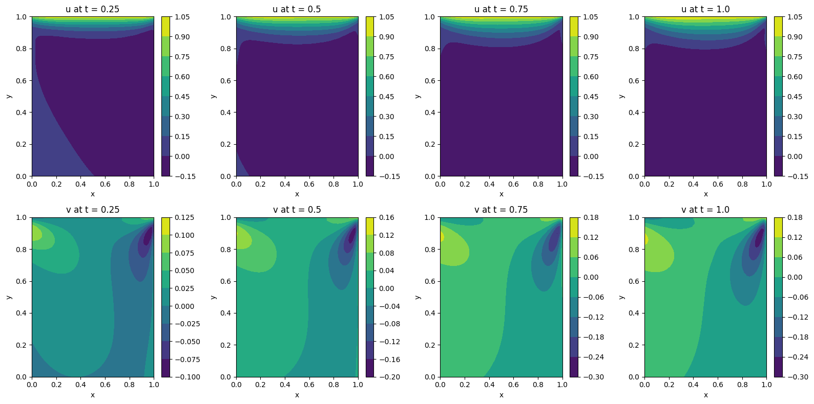
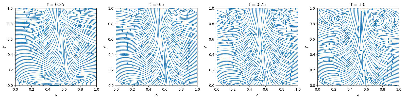
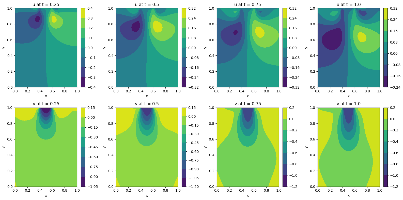
Lid-Driven Square Cavity

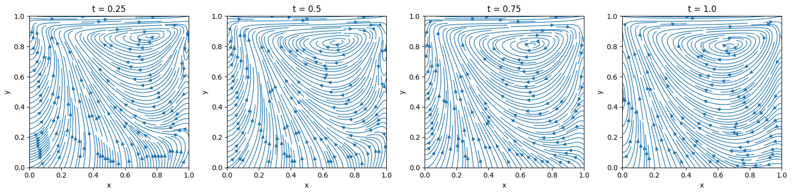
Similarly, the contours of both velocity components (along horizontal and vertical directions) can be plotted at various time intervals for observing changes of each velocity component over time.

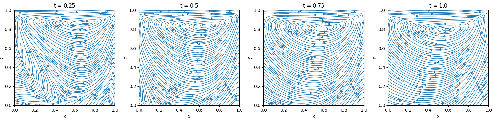
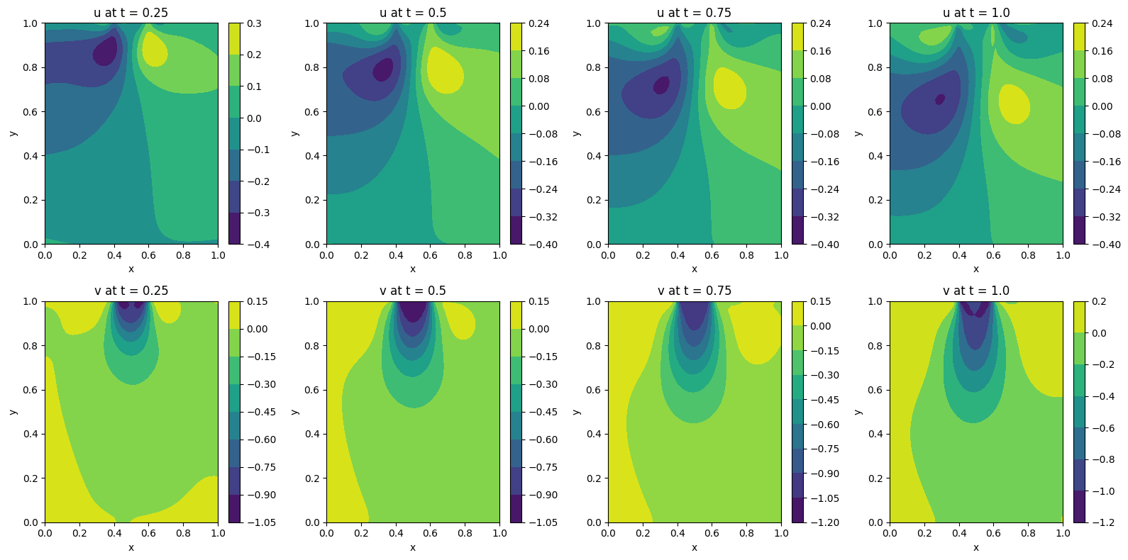
Channel Flow with Jet Impingement

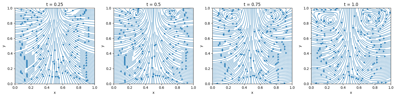
Similarly, the contours of both velocity components (along horizontal and vertical directions) can be plotted at various time intervals for observing changes of each velocity component over time.

• Pressure Poisson Equation can be removed from loss calculation. There are two reasons for this decision.
  • Pressure Poisson Equation is derived from other two equations (continuity and momentum equations).
  • Pressure constraints throughout the network can be enforced in a non-rigid manner.
• The network’s sensitivity to initial conditions has reduced in this method.
• The absence of hard enforcement of BCs in solving other equations suggests that Boundary Encoding Layer is superfluous in the case of 2D Burger’s Equation.

…was the Boundary Encoding Layer even needed in the first place?